Deconvolved Ricker-Wave Site Response
This example starts from a desired surface acceleration and calculates the base motion required to reproduce it through an elastic layered soil profile.
| Application | One-dimensional site response |
| Material behavior | Layered linear elasticity |
| Input workflow | Surface target deconvolved to base motion |
| Analysis | Gravity followed by transient excitation |
| Output | VTKHDF displacement, velocity, and acceleration |
| Execution | Serial |
From A Surface Target To A Base Input
A transfer function describes how a base motion is modified as it propagates through the soil profile. In the frequency domain,
When the desired surface motion is known, deconvolution reverses that mapping:
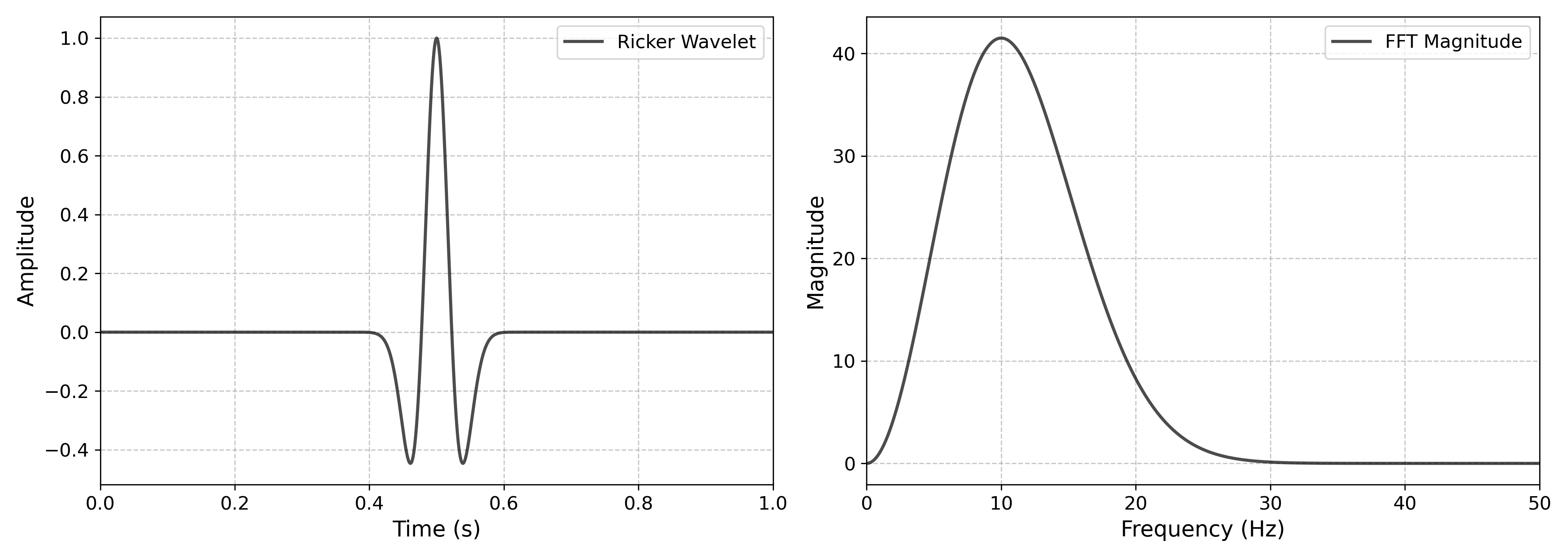
The target in this example is a short Ricker pulse. Femora evaluates the layered-soil transfer function, performs the inverse operation, and adds the quiet lead-in and tail required for a stable time-domain base history.
Deconvolution is preprocessing
The target surface motion is not applied directly to the finite-element model. It defines the response to reproduce. The calculated base motion is the actual uniform-excitation input.
Model
The finite-element model uses the same \(1\text{ m} \times 1\text{ m}\), \(18\text{ m}\)-deep layered profile as the elastic-column example. This keeps the focus on the input-motion workflow rather than introducing a second soil model at the same time.
Worked Workflow
Load the prescribed surface pulse, define the analytical soil and rock profile, and calculate the corresponding base motion.
OUTPUT_DIR.mkdir(parents=True, exist_ok=True)
MOTIONS_OUTPUT_DIR.mkdir(parents=True, exist_ok=True)

motion_directory = motions_dir()
target_surface_motion = TimeHistory.load(
    acc_file=str(motion_directory / "ricker_surface.acc"),
    time_file=str(motion_directory / "ricker_surface.time"),
    unit_in_g=True,
    gravity=GRAVITY,
)

analytical_profile = [
    {
        "h": 2.0,
        "vs": 144.2535646321813,
        "rho": 19.8 * 1_000.0 / GRAVITY,
        "damping": 0.03,
        "damping_type": "rayleigh",
        "f1": 2.76,
        "f2": 13.84,
    },
    {
        "h": 6.0,
        "vs": 196.2675276462639,
        "rho": 19.1 * 1_000.0 / GRAVITY,
        "damping": 0.03,
        "damping_type": "rayleigh",
        "f1": 2.76,
        "f2": 13.84,
    },
    {
        "h": 10.0,
        "vs": 262.5199305117452,
        "rho": 19.9 * 1_000.0 / GRAVITY,
        "damping": 0.03,
        "damping_type": "rayleigh",
        "f1": 2.76,
        "f2": 13.84,
    },
]
rock = {"vs": 8_000.0, "rho": 2_000.0, "damping": 0.0}
transfer_function = TransferFunction(
    soil_profile=analytical_profile,
    rock=rock,
    f_max=50.0,
)
base_motion, aligned_target_motion, _ = transfer_function.deconvolve(
    target_surface_motion,
    return_all=True,
)

base_acceleration_file = MOTIONS_OUTPUT_DIR / "ricker_base.acc"
base_time_file = MOTIONS_OUTPUT_DIR / "ricker_base.time"
target_acceleration_file = MOTIONS_OUTPUT_DIR / "ricker_surface_aligned.acc"
target_time_file = MOTIONS_OUTPUT_DIR / "ricker_surface_aligned.time"

np.savetxt(base_acceleration_file, base_motion.acceleration, fmt="%.10e")
np.savetxt(base_time_file, base_motion.time, fmt="%.10e")
np.savetxt(
    target_acceleration_file,
    aligned_target_motion.acceleration,
    fmt="%.10e",
)
np.savetxt(target_time_file, aligned_target_motion.time, fmt="%.10e")
The layer table creates the materials, brick elements, and mesh parts.
model = Model(
    model_name="deconvolved_ricker_site_response",
    model_path=str(OUTPUT_DIR.resolve()),
)
model.set_results_folder(RESULTS_DIR.resolve().as_posix())

rayleigh_damping = model.damping.frequency_rayleigh(
    user_name="soil_damping",
    f1=2.76,
    f2=13.84,
    damping_factor=0.03,
)
soil_region = model.region.element(
    user_name="soil_column",
    damping=rayleigh_damping,
)

z_bottom = -COLUMN_DEPTH
layer_names = []
for layer in LAYERS:
    density_si = layer["unit_weight"] * 1_000.0 / GRAVITY
    density = density_si / 1_000.0
    young_modulus = (
        2.0
        * layer["shear_modulus"]
        * (1.0 + layer["poisson_ratio"])
        / 1_000.0
    )
    material = model.material.nd.elastic_isotropic(
        user_name=f"{layer['name']}_material",
        E=young_modulus,
        nu=layer["poisson_ratio"],
        rho=density,
    )
    element = model.element.brick.std(
        ndof=3,
        material=material,
        b1=0.0,
        b2=0.0,
        b3=-GRAVITY * density,
    )
    model.meshpart.volume.uniform_rectangular_grid(
        user_name=layer["name"],
        element=element,
        region=soil_region,
        x_min=0.0,
        x_max=COLUMN_WIDTH,
        y_min=0.0,
        y_max=COLUMN_WIDTH,
        z_min=z_bottom,
        z_max=z_bottom + layer["thickness"],
        nx=1,
        ny=1,
        nz=round(layer["thickness"] / layer["element_size"]),
    )
    layer_names.append(layer["name"])
    z_bottom += layer["thickness"]

if abs(z_bottom) > 1.0e-9:
    raise RuntimeError(f"Layer thicknesses terminate at z={z_bottom}, expected z=0")
Assembly forms the column, constraints enforce laminar behavior, and the generated base history becomes a uniform x-direction excitation.
model.assembler.create_section(
    meshparts=layer_names,
    num_partitions=0,
    merge_points=True,
)
model.assembler.assemble(merge_points=True, progress_callback=lambda *_: None)

model.constraint.mp.laminar_boundary(
    bounds=(-COLUMN_DEPTH + 0.1, 0.0),
    dofs=[1, 2, 3],
    direction=3,
)
model.constraint.sp.fix_macro_z_min(dofs=[1, 1, 1], tol=1.0e-6)

base_time_series = model.time_series.path(
    filePath=base_acceleration_file.resolve().as_posix(),
    fileTime=base_time_file.resolve().as_posix(),
    factor=GRAVITY,
)
uniform_excitation = model.pattern.uniform_excitation(
    dof=1,
    time_series=base_time_series,
)
response_recorder = model.recorder.vtkhdf(
    file_base_name="site_response.vtkhdf",
    resp_types=["accel", "disp", "vel"],
    delta_t=DYNAMIC_DT,
)
Femora establishes gravity, resets pseudo-time, and runs the transient Ricker-wave response.
constraint_handler = model.analysis.constraint.transformation()
numberer = model.analysis.numberer.rcm()
system = model.analysis.system.bandgeneral()
algorithm = model.analysis.algorithm.linear()
test = model.analysis.test.normunbalance(tol=1.0e-8, max_iter=10)

newmark_gamma = 0.6
newmark_beta = (newmark_gamma + 0.5) ** 2 / 4.0
gravity_integrator = model.analysis.integrator.newmark(
    gamma=newmark_gamma,
    beta=newmark_beta,
)
dynamic_integrator = model.analysis.integrator.newmark(
    gamma=0.5,
    beta=0.25,
)
gravity_analysis = model.analysis.transient(
    name="gravity",
    constraint_handler=constraint_handler,
    numberer=numberer,
    system=system,
    algorithm=algorithm,
    test=test,
    integrator=gravity_integrator,
    dt=1.0,
    num_steps=30,
)
dynamic_analysis = model.analysis.transient(
    name="ricker_wave",
    constraint_handler=constraint_handler,
    numberer=numberer,
    system=system,
    algorithm=algorithm,
    test=test,
    integrator=dynamic_integrator,
    dt=DYNAMIC_DT,
    final_time=DYNAMIC_FINAL_TIME,
)

model.process.add_step(gravity_analysis, "Establish gravity")
model.process.add_step(uniform_excitation, "Apply the deconvolved base motion")
model.process.add_step(response_recorder, "Record the column response")
model.process.add_step(model.actions.set_time(0.0), "Reset pseudo-time")
model.process.add_step(dynamic_analysis, "Run the Ricker-wave analysis")
Results And Post-Processing
Run the maintained companion after OpenSees completes:
Femora's results API extracts the relative surface acceleration. The post-processor adds the imposed base acceleration to recover the absolute surface motion before comparing it with the target.
def generate_results() -> tuple[Path, ...]:
    """Generate the deconvolution and surface-response comparisons."""
    POSTPROCESS_DIR.mkdir(parents=True, exist_ok=True)
    deconvolution_plot = POSTPROCESS_DIR / "deconvolved-motion.png"
    response_plot = POSTPROCESS_DIR / "surface-response-comparison.png"
    save_deconvolution_plot(deconvolution_plot)

    result_pattern = str(RESULTS_DIR / "site_response*.vtkhdf")
    with fm.results.open(result_pattern) as results:
        surface = results.nearest_point(SURFACE_COORDINATE, tolerance=1.0e-6)
        relative_surface_acceleration = results.point_history(
            "acceleration",
            surface,
            component="x",
        )
        error = save_surface_comparison_plot(
            results.times,
            relative_surface_acceleration,
            response_plot,
        )
    print(f"Normalized surface-response RMS error: {error:.4f}")
    return deconvolution_plot, response_plot


def generate_animations() -> tuple[Path, ...]:
    """Generate the optional amplified response animation."""
    POSTPROCESS_DIR.mkdir(parents=True, exist_ok=True)
    output_file = POSTPROCESS_DIR / "response.mp4"
    result_pattern = str(RESULTS_DIR / "site_response*.vtkhdf")
    with fm.results.open(result_pattern) as results:
        save_response_movie(
            results,
            output_file,
            deformation_scale=15.0,
            stride=10,
            frame_rate=50,
        )
    return (output_file,)
Complete post-processing source
# =============================================================================
# Femora: Fast Efficient Meta-modeling for OpenSees-based Resilience Analysis
# Copyright 2026 Amin Pakzad and Pedro Arduino
# Developed at the UW Geotechnical Lab
# SPDX-License-Identifier: Apache-2.0
# =============================================================================

# femora-colab-source: examples/site_response/layered_elastic_soil_column_postprocess.py

"""Plot and animate the deconvolved Ricker-wave site response."""

from __future__ import annotations

from pathlib import Path

import femora as fm
import matplotlib.pyplot as plt
import numpy as np

if __package__:
    from .layered_elastic_soil_column_postprocess import save_response_movie
else:
    from layered_elastic_soil_column_postprocess import save_response_movie


OUTPUT_DIR = Path("example_outputs") / "deconvolved_ricker_site_response"
RESULTS_DIR = OUTPUT_DIR / "results"
MOTIONS_DIR = OUTPUT_DIR / "motions"
POSTPROCESS_DIR = OUTPUT_DIR / "post_processing"

GRAVITY = 9.81
SURFACE_COORDINATE = np.array([0.0, 0.0, 0.0])


def _load_motion(stem: str) -> tuple[np.ndarray, np.ndarray]:
    """Load one generated acceleration history from the example output."""
    return (
        np.loadtxt(MOTIONS_DIR / f"{stem}.time"),
        np.loadtxt(MOTIONS_DIR / f"{stem}.acc"),
    )


def save_deconvolution_plot(output_file: Path) -> None:
    """Plot the prescribed surface pulse and calculated base motion."""
    target_time, target_acceleration = _load_motion("ricker_surface_aligned")
    base_time, base_acceleration = _load_motion("ricker_base")

    figure, axes = plt.subplots(
        2,
        1,
        figsize=(9.0, 5.8),
        sharex=True,
        constrained_layout=True,
    )
    axes[0].plot(target_time, target_acceleration, color="#b65f3a", linewidth=1.4)
    axes[0].set_title("Target surface motion", loc="left")
    axes[1].plot(base_time, base_acceleration, color="#315c6d", linewidth=1.3)
    axes[1].set_title("Deconvolved base motion", loc="left")
    axes[1].set_xlabel("Time (s)")
    for axis in axes:
        axis.set_ylabel("Acceleration (g)")
        axis.grid(alpha=0.25)
        axis.spines[["top", "right"]].set_visible(False)
    figure.savefig(output_file, dpi=180)
    plt.close(figure)


def save_surface_comparison_plot(
    response_time: np.ndarray,
    relative_surface_acceleration: np.ndarray,
    output_file: Path,
) -> float:
    """Compare the absolute numerical response with the target surface pulse."""
    target_time, target_acceleration_g = _load_motion("ricker_surface_aligned")
    base_time, base_acceleration_g = _load_motion("ricker_base")

    base_acceleration = np.interp(
        response_time,
        base_time,
        base_acceleration_g * GRAVITY,
    )
    numerical_surface_g = (
        relative_surface_acceleration + base_acceleration
    ) / GRAVITY
    target_on_response = np.interp(
        response_time,
        target_time,
        target_acceleration_g,
    )
    active = response_time <= target_time[-1]
    difference = numerical_surface_g[active] - target_on_response[active]
    reference_rms = float(np.sqrt(np.mean(target_on_response[active] ** 2)))
    normalized_rms_error = float(np.sqrt(np.mean(difference**2)) / reference_rms)

    figure, axis = plt.subplots(figsize=(9.0, 4.8), constrained_layout=True)
    axis.plot(
        response_time[active],
        target_on_response[active],
        color="#b65f3a",
        linewidth=1.6,
        linestyle="--",
        label="Target surface",
    )
    axis.plot(
        response_time[active],
        numerical_surface_g[active],
        color="#315c6d",
        linewidth=1.25,
        label="Numerical surface",
    )
    axis.set(xlabel="Time (s)", ylabel="Acceleration (g)")
    axis.grid(alpha=0.25)
    axis.legend(frameon=False)
    axis.spines[["top", "right"]].set_visible(False)
    axis.text(
        0.99,
        0.04,
        f"Normalized RMS error: {normalized_rms_error:.3f}",
        ha="right",
        va="bottom",
        transform=axis.transAxes,
    )
    figure.savefig(output_file, dpi=180)
    plt.close(figure)
    return normalized_rms_error


def generate_results() -> tuple[Path, ...]:
    """Generate the deconvolution and surface-response comparisons."""
    POSTPROCESS_DIR.mkdir(parents=True, exist_ok=True)
    deconvolution_plot = POSTPROCESS_DIR / "deconvolved-motion.png"
    response_plot = POSTPROCESS_DIR / "surface-response-comparison.png"
    save_deconvolution_plot(deconvolution_plot)

    result_pattern = str(RESULTS_DIR / "site_response*.vtkhdf")
    with fm.results.open(result_pattern) as results:
        surface = results.nearest_point(SURFACE_COORDINATE, tolerance=1.0e-6)
        relative_surface_acceleration = results.point_history(
            "acceleration",
            surface,
            component="x",
        )
        error = save_surface_comparison_plot(
            results.times,
            relative_surface_acceleration,
            response_plot,
        )
    print(f"Normalized surface-response RMS error: {error:.4f}")
    return deconvolution_plot, response_plot


def generate_animations() -> tuple[Path, ...]:
    """Generate the optional amplified response animation."""
    POSTPROCESS_DIR.mkdir(parents=True, exist_ok=True)
    output_file = POSTPROCESS_DIR / "response.mp4"
    result_pattern = str(RESULTS_DIR / "site_response*.vtkhdf")
    with fm.results.open(result_pattern) as results:
        save_response_movie(
            results,
            output_file,
            deformation_scale=15.0,
            stride=10,
            frame_rate=50,
        )
    return (output_file,)


def main() -> None:
    """Generate all documented post-processing outputs."""
    generated = (*generate_results(), *generate_animations())
    print("Post-processing outputs:")
    for output in generated:
        print(f"  {output.resolve()}")


if __name__ == "__main__":
    main()
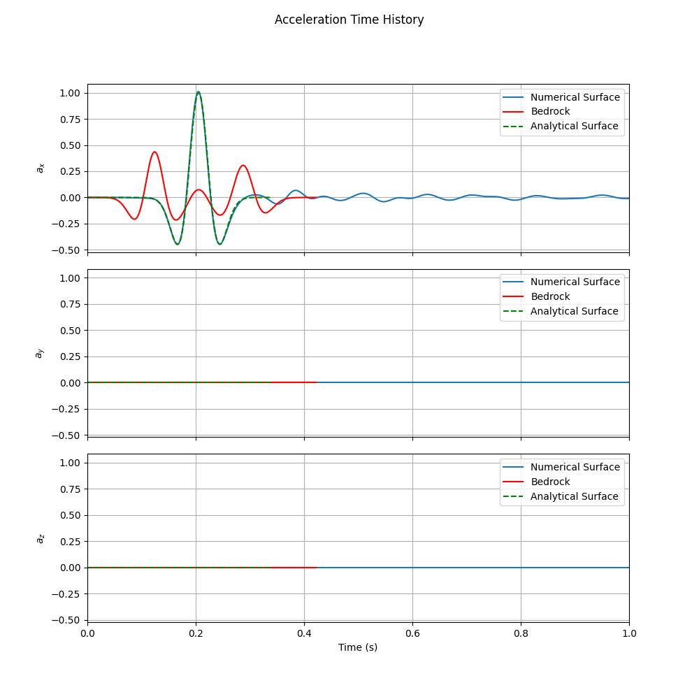
The numerical absolute surface acceleration closely follows the prescribed Ricker pulse. The deconvolved base motion is also shown to make the complete inverse-and-forward workflow visible.
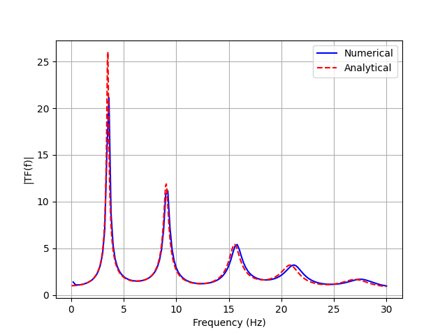
The numerical surface-to-base amplification reproduces the analytical layered-profile transfer function over the frequency range excited by the Ricker pulse.
The optional animation uses the same VTKHDF response to show amplified horizontal deformation through the three physical soil strata.
Result provenance
These reference figures and the animation were produced by the validated legacy Example 4 benchmark. The migrated example preserves its profile, deconvolution input, integration parameters, and output quantities. Running the maintained source regenerates the same result types through the current Femora APIs.
Run The Example
Use Open in Colab to execute preprocessing, model construction, OpenSees, and static post-processing in sequence. Locally, export the model with:
To execute OpenSees as well:
$env:FEMORA_OPENSEES = "D:\path\to\OpenSees.exe"
python examples/site_response/deconvolved_ricker_site_response.py
The default output directory contains the generated base and aligned target motions, exported Tcl model, solver results, and post-processing products.
Complete source
# =============================================================================
# Femora: Fast Efficient Meta-modeling for OpenSees-based Resilience Analysis
# Copyright 2026 Amin Pakzad and Pedro Arduino
# Developed at the UW Geotechnical Lab
# SPDX-License-Identifier: Apache-2.0
# =============================================================================

# femora-colab-input: examples/inputs/motions/ricker_surface.acc
# femora-colab-input: examples/inputs/motions/ricker_surface.time
# femora-postprocess: examples/site_response/deconvolved_ricker_site_response_postprocess.py

# %% [markdown]
# # Deconvolved Ricker-Wave Site Response
#
# Start from a target surface acceleration, deconvolve it through an elastic
# layered profile, and apply the resulting base motion to a Femora model.

# %%
"""Run elastic site response using a deconvolved Ricker-wave base motion."""

from __future__ import annotations

import os
from pathlib import Path

import numpy as np

from femora import Model, runtime
from femora.tools.transferFunction import TimeHistory, TransferFunction
from femora.utils.paths import motions_dir


OUTPUT_DIR = Path("example_outputs") / "deconvolved_ricker_site_response"
RESULTS_DIR = OUTPUT_DIR / "results"
MOTIONS_OUTPUT_DIR = OUTPUT_DIR / "motions"
OPENSEES = os.environ.get("FEMORA_OPENSEES")
PLOT_MODEL = False

COLUMN_WIDTH = 1.0
COLUMN_DEPTH = 18.0
GRAVITY = 9.81
DYNAMIC_DT = 0.001
DYNAMIC_FINAL_TIME = 5.0

LAYERS = [
    {
        "name": "dense_ottawa_lower",
        "shear_modulus": 145.0e6,
        "unit_weight": 19.9,
        "poisson_ratio": 0.3,
        "thickness": 2.6,
        "element_size": 1.3,
    },
    {
        "name": "dense_ottawa_middle",
        "shear_modulus": 145.0e6,
        "unit_weight": 19.9,
        "poisson_ratio": 0.3,
        "thickness": 2.4,
        "element_size": 1.2,
    },
    {
        "name": "dense_ottawa_upper",
        "shear_modulus": 145.0e6,
        "unit_weight": 19.9,
        "poisson_ratio": 0.3,
        "thickness": 5.0,
        "element_size": 1.0,
    },
    {
        "name": "loose_ottawa",
        "shear_modulus": 75.0e6,
        "unit_weight": 19.1,
        "poisson_ratio": 0.3,
        "thickness": 6.0,
        "element_size": 0.5,
    },
    {
        "name": "dense_monterey",
        "shear_modulus": 42.0e6,
        "unit_weight": 19.8,
        "poisson_ratio": 0.3,
        "thickness": 2.0,
        "element_size": 0.5,
    },
]


# %% [markdown]
# ## Deconvolve the target surface motion
#
# The analytical profile maps base motion to surface motion. Deconvolution
# applies the inverse of that transfer function to obtain the required input.

# %%
OUTPUT_DIR.mkdir(parents=True, exist_ok=True)
MOTIONS_OUTPUT_DIR.mkdir(parents=True, exist_ok=True)

motion_directory = motions_dir()
target_surface_motion = TimeHistory.load(
    acc_file=str(motion_directory / "ricker_surface.acc"),
    time_file=str(motion_directory / "ricker_surface.time"),
    unit_in_g=True,
    gravity=GRAVITY,
)

analytical_profile = [
    {
        "h": 2.0,
        "vs": 144.2535646321813,
        "rho": 19.8 * 1_000.0 / GRAVITY,
        "damping": 0.03,
        "damping_type": "rayleigh",
        "f1": 2.76,
        "f2": 13.84,
    },
    {
        "h": 6.0,
        "vs": 196.2675276462639,
        "rho": 19.1 * 1_000.0 / GRAVITY,
        "damping": 0.03,
        "damping_type": "rayleigh",
        "f1": 2.76,
        "f2": 13.84,
    },
    {
        "h": 10.0,
        "vs": 262.5199305117452,
        "rho": 19.9 * 1_000.0 / GRAVITY,
        "damping": 0.03,
        "damping_type": "rayleigh",
        "f1": 2.76,
        "f2": 13.84,
    },
]
rock = {"vs": 8_000.0, "rho": 2_000.0, "damping": 0.0}
transfer_function = TransferFunction(
    soil_profile=analytical_profile,
    rock=rock,
    f_max=50.0,
)
base_motion, aligned_target_motion, _ = transfer_function.deconvolve(
    target_surface_motion,
    return_all=True,
)

base_acceleration_file = MOTIONS_OUTPUT_DIR / "ricker_base.acc"
base_time_file = MOTIONS_OUTPUT_DIR / "ricker_base.time"
target_acceleration_file = MOTIONS_OUTPUT_DIR / "ricker_surface_aligned.acc"
target_time_file = MOTIONS_OUTPUT_DIR / "ricker_surface_aligned.time"

np.savetxt(base_acceleration_file, base_motion.acceleration, fmt="%.10e")
np.savetxt(base_time_file, base_motion.time, fmt="%.10e")
np.savetxt(
    target_acceleration_file,
    aligned_target_motion.acceleration,
    fmt="%.10e",
)
np.savetxt(target_time_file, aligned_target_motion.time, fmt="%.10e")


# %% [markdown]
# ## Build the layered column

# %%
model = Model(
    model_name="deconvolved_ricker_site_response",
    model_path=str(OUTPUT_DIR.resolve()),
)
model.set_results_folder(RESULTS_DIR.resolve().as_posix())

rayleigh_damping = model.damping.frequency_rayleigh(
    user_name="soil_damping",
    f1=2.76,
    f2=13.84,
    damping_factor=0.03,
)
soil_region = model.region.element(
    user_name="soil_column",
    damping=rayleigh_damping,
)

z_bottom = -COLUMN_DEPTH
layer_names = []
for layer in LAYERS:
    density_si = layer["unit_weight"] * 1_000.0 / GRAVITY
    density = density_si / 1_000.0
    young_modulus = (
        2.0
        * layer["shear_modulus"]
        * (1.0 + layer["poisson_ratio"])
        / 1_000.0
    )
    material = model.material.nd.elastic_isotropic(
        user_name=f"{layer['name']}_material",
        E=young_modulus,
        nu=layer["poisson_ratio"],
        rho=density,
    )
    element = model.element.brick.std(
        ndof=3,
        material=material,
        b1=0.0,
        b2=0.0,
        b3=-GRAVITY * density,
    )
    model.meshpart.volume.uniform_rectangular_grid(
        user_name=layer["name"],
        element=element,
        region=soil_region,
        x_min=0.0,
        x_max=COLUMN_WIDTH,
        y_min=0.0,
        y_max=COLUMN_WIDTH,
        z_min=z_bottom,
        z_max=z_bottom + layer["thickness"],
        nx=1,
        ny=1,
        nz=round(layer["thickness"] / layer["element_size"]),
    )
    layer_names.append(layer["name"])
    z_bottom += layer["thickness"]

if abs(z_bottom) > 1.0e-9:
    raise RuntimeError(f"Layer thicknesses terminate at z={z_bottom}, expected z=0")


# %% [markdown]
# ## Assemble, constrain, and excite the model

# %%
model.assembler.create_section(
    meshparts=layer_names,
    num_partitions=0,
    merge_points=True,
)
model.assembler.assemble(merge_points=True, progress_callback=lambda *_: None)

model.constraint.mp.laminar_boundary(
    bounds=(-COLUMN_DEPTH + 0.1, 0.0),
    dofs=[1, 2, 3],
    direction=3,
)
model.constraint.sp.fix_macro_z_min(dofs=[1, 1, 1], tol=1.0e-6)

base_time_series = model.time_series.path(
    filePath=base_acceleration_file.resolve().as_posix(),
    fileTime=base_time_file.resolve().as_posix(),
    factor=GRAVITY,
)
uniform_excitation = model.pattern.uniform_excitation(
    dof=1,
    time_series=base_time_series,
)
response_recorder = model.recorder.vtkhdf(
    file_base_name="site_response.vtkhdf",
    resp_types=["accel", "disp", "vel"],
    delta_t=DYNAMIC_DT,
)


# %% [markdown]
# ## Define and run the staged analysis

# %%
constraint_handler = model.analysis.constraint.transformation()
numberer = model.analysis.numberer.rcm()
system = model.analysis.system.bandgeneral()
algorithm = model.analysis.algorithm.linear()
test = model.analysis.test.normunbalance(tol=1.0e-8, max_iter=10)

newmark_gamma = 0.6
newmark_beta = (newmark_gamma + 0.5) ** 2 / 4.0
gravity_integrator = model.analysis.integrator.newmark(
    gamma=newmark_gamma,
    beta=newmark_beta,
)
dynamic_integrator = model.analysis.integrator.newmark(
    gamma=0.5,
    beta=0.25,
)
gravity_analysis = model.analysis.transient(
    name="gravity",
    constraint_handler=constraint_handler,
    numberer=numberer,
    system=system,
    algorithm=algorithm,
    test=test,
    integrator=gravity_integrator,
    dt=1.0,
    num_steps=30,
)
dynamic_analysis = model.analysis.transient(
    name="ricker_wave",
    constraint_handler=constraint_handler,
    numberer=numberer,
    system=system,
    algorithm=algorithm,
    test=test,
    integrator=dynamic_integrator,
    dt=DYNAMIC_DT,
    final_time=DYNAMIC_FINAL_TIME,
)

model.process.add_step(gravity_analysis, "Establish gravity")
model.process.add_step(uniform_excitation, "Apply the deconvolved base motion")
model.process.add_step(response_recorder, "Record the column response")
model.process.add_step(model.actions.set_time(0.0), "Reset pseudo-time")
model.process.add_step(dynamic_analysis, "Run the Ricker-wave analysis")


# %% [markdown]
# ## Export and optionally execute

# %%
tcl_file = OUTPUT_DIR / "deconvolved_ricker_site_response.tcl"
model.export_to_tcl(
    filename=str(tcl_file.resolve()),
    progress_callback=lambda *_: None,
)

print("\nDeconvolved Ricker-wave site response")
print(f"  Nodes:          {model.assembled_mesh.n_points}")
print(f"  Elements:       {model.assembled_mesh.n_cells}")
print(f"  Base samples:   {base_motion.time.size}")
print(f"  Base motion:    {base_acceleration_file.resolve()}")
print(f"  Tcl model:      {tcl_file.resolve()}")

if OPENSEES is None:
    print("  Solver:         not run (set FEMORA_OPENSEES to run OpenSees)")
else:
    runtime.run(
        tcl_file,
        executable=OPENSEES,
        cwd=OUTPUT_DIR.resolve(),
    )
    print("  Solver:         completed")


# %% [markdown]
# ## Optional visualization

# %%
if PLOT_MODEL:
    model.assembler.plot(show_edges=True, scalars="MaterialTag")