Layered Elastic Soil Column
This example models the one-dimensional response of a five-layer elastic soil profile subjected to a horizontal frequency-sweep excitation.
| Application | One-dimensional site response |
| Material behavior | Layered linear elasticity |
| Analysis | Gravity followed by transient excitation |
| Boundary condition | Laminar column with a fixed base |
| Output | VTKHDF displacement, velocity, and acceleration |
| Execution | Serial |
Model
The \(1\text{ m} \times 1\text{ m}\) column extends from \(z=-18\text{ m}\) to the ground surface. Each color identifies a material layer. Nodes at each elevation are tied with laminar constraints, so the narrow 3D mesh reproduces one-dimensional shear-wave propagation while retaining brick elements.
Applied motion
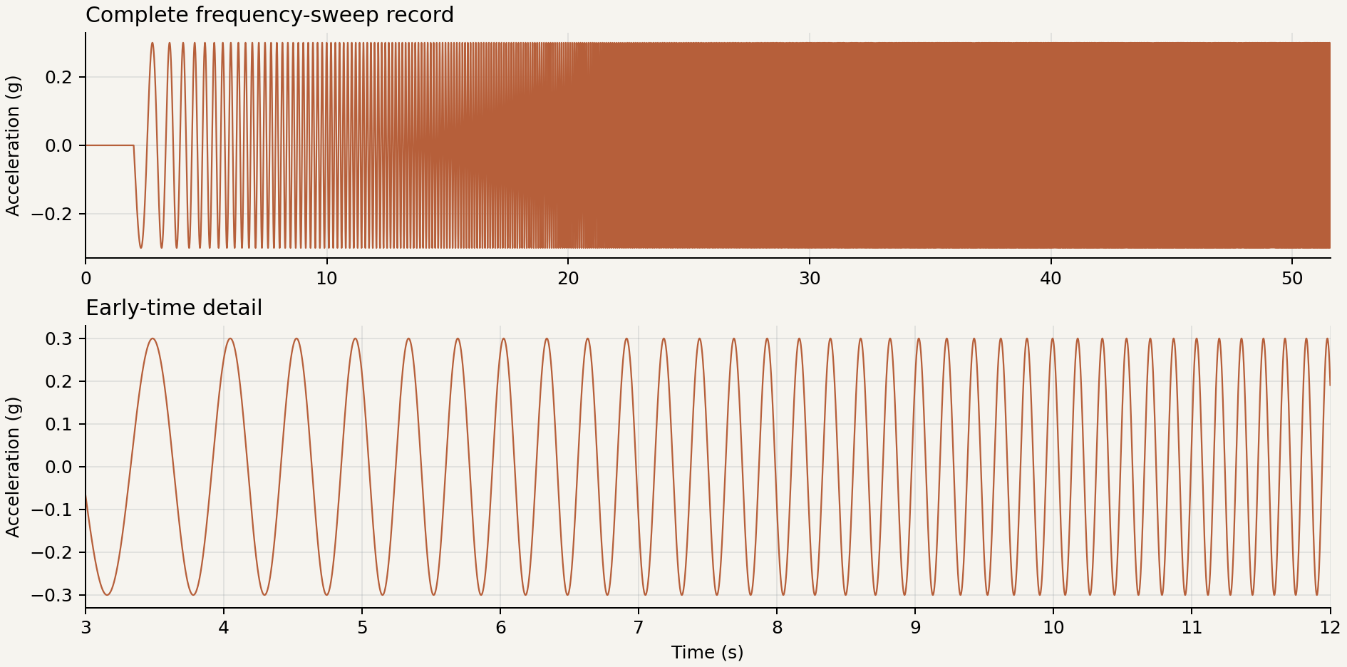
The base acceleration is a frequency sweep whose frequency increases with time. This makes the model pass through a broad frequency range in one analysis and exposes the profile's principal amplification peaks.
Soil Profile
| Layer | Thickness (m) | \(G\) (MPa) | Unit weight (kN/m\(^3\)) | \(V_s\) (m/s) | Element height (m) |
|---|---|---|---|---|---|
| Dense Ottawa, lower | 2.6 | 145 | 19.9 | 267.36 | 1.3 |
| Dense Ottawa, middle | 2.4 | 145 | 19.9 | 267.36 | 1.2 |
| Dense Ottawa, upper | 5.0 | 145 | 19.9 | 267.36 | 1.0 |
| Loose Ottawa | 6.0 | 75 | 19.1 | 196.27 | 0.5 |
| Dense Monterey | 2.0 | 42 | 19.8 | 144.25 | 0.5 |
The source uses a consistent kN-m-s unit system. It converts the tabulated SI stiffness and mass density before creating each Femora material.
Key Model Definitions
Each layer creates its own material, brick element, and mesh part from the profile table.
z_bottom = -COLUMN_DEPTH
layer_names = []

for layer in LAYERS:
    name = layer["name"]
    shear_modulus = layer["shear_modulus"]
    unit_weight = layer["unit_weight"]
    poisson_ratio = layer["poisson_ratio"]
    thickness = layer["thickness"]
    element_size = layer["element_size"]

    density_si = unit_weight * 1_000.0 / GRAVITY
    shear_velocity = (shear_modulus / density_si) ** 0.5
    young_modulus_si = 2.0 * shear_modulus * (1.0 + poisson_ratio)

    # Convert Pa to kPa and kg/m^3 to Mg/m^3 for the kN-m-s unit system.
    young_modulus = young_modulus_si / 1_000.0
    density = density_si / 1_000.0

    print(f"{name:24s} Vs = {shear_velocity:7.2f} m/s")

    material = model.material.nd.elastic_isotropic(
        user_name=f"{name}_material",
        E=young_modulus,
        nu=poisson_ratio,
        rho=density,
    )
    element = model.element.brick.std(
        ndof=3,
        material=material,
        b1=0.0,
        b2=0.0,
        b3=-GRAVITY * density,
    )

    number_of_elements = round(thickness / element_size)
    model.meshpart.volume.uniform_rectangular_grid(
        user_name=name,
        element=element,
        region=soil_region,
        x_min=0.0,
        x_max=COLUMN_WIDTH,
        y_min=0.0,
        y_max=COLUMN_WIDTH,
        z_min=z_bottom,
        z_max=z_bottom + thickness,
        nx=1,
        ny=1,
        nz=number_of_elements,
    )
    layer_names.append(name)
    z_bottom += thickness

if abs(z_bottom) > 1.0e-9:
    raise RuntimeError(f"Layer thicknesses terminate at z={z_bottom}, expected z=0")
Assembly joins the independently generated layers. Laminar constraints tie equal-elevation boundary nodes, and the base restrains all translations.
model.assembler.create_section(
    meshparts=layer_names,
    num_partitions=0,
    merge_points=True,
)
model.assembler.assemble(merge_points=True, progress_callback=lambda *_: None)

model.constraint.mp.laminar_boundary(
    bounds=(-COLUMN_DEPTH + 0.1, 0.0),
    dofs=[1, 2, 3],
    direction=3,
)
model.constraint.sp.fix_macro_z_min(
    dofs=[1, 1, 1],
    tol=1.0e-6,
)
A nonuniform Path time series drives a uniform x-direction excitation. The VTKHDF recorder writes the full transient field response every (0.01) s.
motion_directory = motions_dir()
excitation = model.time_series.path(
    filePath=(motion_directory / "FrequencySweep.acc").resolve().as_posix(),
    fileTime=(motion_directory / "FrequencySweep.time").resolve().as_posix(),
    factor=MOTION_SCALE,
)
uniform_excitation = model.pattern.uniform_excitation(
    dof=1,
    time_series=excitation,
)

response_recorder = model.recorder.vtkhdf(
    file_base_name="site_response.vtkhdf",
    resp_types=["accel", "disp", "vel"],
    delta_t=0.01,
)
The process establishes gravity, activates the excitation and recorder, resets pseudo-time, and then runs the transient response.
constraint_handler = model.analysis.constraint.transformation()
numberer = model.analysis.numberer.rcm()
system = model.analysis.system.bandgeneral()
algorithm = model.analysis.algorithm.linear()
test = model.analysis.test.normunbalance(tol=1.0e-8, max_iter=10)

newmark_gamma = 0.6
newmark_beta = (newmark_gamma + 0.5) ** 2 / 4.0
integrator = model.analysis.integrator.newmark(
    gamma=newmark_gamma,
    beta=newmark_beta,
)

gravity_analysis = model.analysis.transient(
    name="gravity",
    constraint_handler=constraint_handler,
    numberer=numberer,
    system=system,
    algorithm=algorithm,
    test=test,
    integrator=integrator,
    dt=1.0,
    num_steps=30,
)
dynamic_analysis = model.analysis.transient(
    name="frequency_sweep",
    constraint_handler=constraint_handler,
    numberer=numberer,
    system=system,
    algorithm=algorithm,
    test=test,
    integrator=integrator,
    dt=DYNAMIC_DT,
    final_time=DYNAMIC_FINAL_TIME,
)

model.process.add_step(gravity_analysis, "Establish gravity")
model.process.add_step(uniform_excitation, "Apply the base excitation")
model.process.add_step(response_recorder, "Record the column response")
model.process.add_step(model.actions.set_time(0.0), "Reset pseudo-time")
model.process.add_step(dynamic_analysis, "Run the site-response analysis")
Results And Post-Processing
The post-processing script reads the recorded VTKHDF response and generates both results shown here.
Run this file after OpenSees completes the analysis:
The workflow below comes directly from the maintained post-processing file. Femora handles result discovery, history extraction, partitioned fields, and animation frames; the example retains its engineering choices.
def generate_results() -> tuple[Path, ...]:
    """Generate inexpensive plots intended for normal notebook execution."""
    POSTPROCESS_DIR.mkdir(parents=True, exist_ok=True)
    result_pattern = str(RESULTS_DIR / "site_response*.vtkhdf")
    with fm.results.open(result_pattern) as results:
        surface = results.nearest_point(
            SURFACE_COORDINATE,
            tolerance=1.0e-6,
        )
        surface_acceleration = results.point_history(
            "acceleration",
            surface,
            component="x",
        )

        numerical_frequency, numerical_tf = compute_numerical_transfer_function(
            results.times,
            surface_acceleration,
        )
        analytical_frequency, analytical_tf = compute_analytical_transfer_function()
        save_transfer_function_plot(
            numerical_frequency,
            numerical_tf,
            analytical_frequency,
            analytical_tf,
            POSTPROCESS_DIR / "transfer-function-comparison.png",
        )
    return (POSTPROCESS_DIR / "transfer-function-comparison.png",)


def generate_animations() -> tuple[Path, ...]:
    """Generate optional animations that can take substantially longer."""
    POSTPROCESS_DIR.mkdir(parents=True, exist_ok=True)
    result_pattern = str(RESULTS_DIR / "site_response*.vtkhdf")
    with fm.results.open(result_pattern) as results:
        save_response_movie(results, POSTPROCESS_DIR / "response.mp4")
    return (POSTPROCESS_DIR / "response.mp4",)
Complete post-processing source
# =============================================================================
# Femora: Fast Efficient Meta-modeling for OpenSees-based Resilience Analysis
# Copyright 2026 Amin Pakzad and Pedro Arduino
# Developed at the UW Geotechnical Lab
# SPDX-License-Identifier: Apache-2.0
# =============================================================================

"""Plot and animate the layered elastic soil-column response."""

from __future__ import annotations

from pathlib import Path

import femora as fm
import matplotlib.pyplot as plt
import numpy as np

from femora.tools.transferFunction import TransferFunction
from femora.utils.paths import motions_dir


OUTPUT_DIR = Path("example_outputs") / "layered_elastic_soil_column"
RESULTS_DIR = OUTPUT_DIR / "results"
POSTPROCESS_DIR = OUTPUT_DIR / "post_processing"

GRAVITY = 9.81
SURFACE_COORDINATE = np.array([0.0, 0.0, 0.0])
MAX_FREQUENCY = 22.0
DEFORMATION_SCALE = 15.0
MOVIE_STRIDE = 2
MOVIE_FRAME_RATE = 50


def compute_numerical_transfer_function(
    response_time: np.ndarray,
    relative_surface_acceleration: np.ndarray,
) -> tuple[np.ndarray, np.ndarray]:
    """Calculate the absolute surface-to-base transfer function."""
    motion_directory = motions_dir()
    input_time = np.loadtxt(motion_directory / "FrequencySweep.time")
    input_acceleration = (
        np.loadtxt(motion_directory / "FrequencySweep.acc") * GRAVITY
    )
    base_acceleration = np.interp(response_time, input_time, input_acceleration)
    absolute_surface_acceleration = relative_surface_acceleration + base_acceleration

    dt = float(np.mean(np.diff(response_time)))
    frequency = np.fft.rfftfreq(response_time.size, d=dt)
    base_spectrum = np.fft.rfft(base_acceleration)
    surface_spectrum = np.fft.rfft(absolute_surface_acceleration)
    transfer_function = np.divide(
        surface_spectrum,
        base_spectrum,
        out=np.full_like(surface_spectrum, np.nan),
        where=np.abs(base_spectrum) > np.finfo(float).eps,
    )
    return frequency, transfer_function


def compute_analytical_transfer_function() -> tuple[np.ndarray, np.ndarray]:
    """Calculate the analytical response for the three physical strata."""
    soil_profile = [
        {
            "h": 2.0,
            "vs": 144.2535646321813,
            "rho": 19.8 * 1_000.0 / GRAVITY,
            "damping": 0.03,
            "damping_type": "rayleigh",
            "f1": 2.76,
            "f2": 13.84,
        },
        {
            "h": 6.0,
            "vs": 196.2675276462639,
            "rho": 19.1 * 1_000.0 / GRAVITY,
            "damping": 0.03,
            "damping_type": "rayleigh",
            "f1": 2.76,
            "f2": 13.84,
        },
        {
            "h": 10.0,
            "vs": 267.3633200780943,
            "rho": 19.9 * 1_000.0 / GRAVITY,
            "damping": 0.03,
            "damping_type": "rayleigh",
            "f1": 2.76,
            "f2": 13.84,
        },
    ]
    rock = {"vs": 8_000.0, "rho": 2_000.0, "damping": 0.0}
    frequency, transfer_function, _ = TransferFunction(
        soil_profile=soil_profile,
        rock=rock,
        f_max=MAX_FREQUENCY,
    ).compute()
    return frequency, transfer_function


def save_transfer_function_plot(
    numerical_frequency: np.ndarray,
    numerical_transfer_function: np.ndarray,
    analytical_frequency: np.ndarray,
    analytical_transfer_function: np.ndarray,
    output_file: Path,
) -> None:
    """Save the numerical and analytical amplification comparison."""
    frequency_mask = (
        (numerical_frequency > 0.0) & (numerical_frequency <= MAX_FREQUENCY)
    )
    figure, axis = plt.subplots(figsize=(9.0, 4.8), constrained_layout=True)
    axis.plot(
        numerical_frequency[frequency_mask],
        np.abs(numerical_transfer_function[frequency_mask]),
        color="#315c6d",
        linewidth=1.7,
        label="Numerical",
    )
    axis.plot(
        analytical_frequency,
        np.abs(analytical_transfer_function),
        color="#b65f3a",
        linewidth=1.5,
        linestyle="--",
        label="Analytical",
    )
    axis.set(xlabel="Frequency (Hz)", ylabel="Amplification, |TF(f)|")
    axis.set_xlim(0.0, MAX_FREQUENCY)
    axis.grid(alpha=0.25)
    axis.legend(frameon=False)
    figure.savefig(output_file, dpi=180)
    plt.close(figure)


def save_response_movie(
    results: fm.results.ResultSet,
    output_file: Path,
    *,
    deformation_scale: float = DEFORMATION_SCALE,
    stride: int = MOVIE_STRIDE,
    frame_rate: int = MOVIE_FRAME_RATE,
) -> None:
    """Save an amplified deformation animation colored by physical stratum."""
    for partition in range(results.number_of_partitions):
        mesh = results.mesh(partition)
        cell_elevation = mesh.cell_centers().points[:, 2]
        material_layer = np.full(mesh.n_cells, 2, dtype=int)
        material_layer[cell_elevation < -2.0] = 1
        material_layer[cell_elevation < -8.0] = 0
        mesh.cell_data["Physical layer"] = material_layer

    renderer = results.deformation_renderer()
    renderer.deform_by("displacement", scale=deformation_scale)
    renderer.color_by(
        "Physical layer",
        location="cell",
        categories=True,
        cmap=["#315c6d", "#c59652", "#b65f3a"],
        show_scalar_bar=False,
    )
    renderer.set_view(
        background="#f6f4ef",
    )
    renderer.write(
        output_file,
        stride=stride,
        frame_rate=frame_rate,
    )


def generate_results() -> tuple[Path, ...]:
    """Generate inexpensive plots intended for normal notebook execution."""
    POSTPROCESS_DIR.mkdir(parents=True, exist_ok=True)
    result_pattern = str(RESULTS_DIR / "site_response*.vtkhdf")
    with fm.results.open(result_pattern) as results:
        surface = results.nearest_point(
            SURFACE_COORDINATE,
            tolerance=1.0e-6,
        )
        surface_acceleration = results.point_history(
            "acceleration",
            surface,
            component="x",
        )

        numerical_frequency, numerical_tf = compute_numerical_transfer_function(
            results.times,
            surface_acceleration,
        )
        analytical_frequency, analytical_tf = compute_analytical_transfer_function()
        save_transfer_function_plot(
            numerical_frequency,
            numerical_tf,
            analytical_frequency,
            analytical_tf,
            POSTPROCESS_DIR / "transfer-function-comparison.png",
        )
    return (POSTPROCESS_DIR / "transfer-function-comparison.png",)


def generate_animations() -> tuple[Path, ...]:
    """Generate optional animations that can take substantially longer."""
    POSTPROCESS_DIR.mkdir(parents=True, exist_ok=True)
    result_pattern = str(RESULTS_DIR / "site_response*.vtkhdf")
    with fm.results.open(result_pattern) as results:
        save_response_movie(results, POSTPROCESS_DIR / "response.mp4")
    return (POSTPROCESS_DIR / "response.mp4",)


def main() -> None:
    """Generate all documented post-processing outputs."""
    generated = (*generate_results(), *generate_animations())
    print("Post-processing outputs:")
    for output in generated:
        print(f"  {output.resolve()}")


if __name__ == "__main__":
    main()
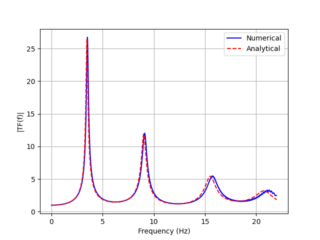
The numerical surface-to-base amplification follows the analytical layered-soil transfer function, including the principal resonance peaks.
The animation shows the amplified horizontal deformation during the frequency sweep. Colors identify the three physical soil strata; the first three mesh parts form the single 10 m Dense Ottawa stratum.
Run The Example
Use Open in Colab to run the complete model in a prepared browser runtime. The generated setup cell installs Femora, configures OpenSees, and downloads only the two required motion files.
For a local export:
To execute OpenSees as well:
$env:FEMORA_OPENSEES = "D:\path\to\OpenSees.exe"
python examples/site_response/layered_elastic_soil_column.py
A local export reports:
The default example_outputs/layered_elastic_soil_column/ directory contains
the OpenSees Tcl model and, after solver execution, the recorded VTKHDF
response.
Complete source
# =============================================================================
# Femora: Fast Efficient Meta-modeling for OpenSees-based Resilience Analysis
# Copyright 2026 Amin Pakzad and Pedro Arduino
# Developed at the UW Geotechnical Lab
# SPDX-License-Identifier: Apache-2.0
# =============================================================================

# femora-colab-input: examples/inputs/motions/FrequencySweep.acc
# femora-colab-input: examples/inputs/motions/FrequencySweep.time
# femora-postprocess: examples/site_response/layered_elastic_soil_column_postprocess.py

# %% [markdown]
# # Layered Elastic Soil Column
#
# Build a five-mesh-part, three-stratum soil column, apply a frequency-sweep
# base excitation, and record the transient response in VTKHDF format.

# %%
"""Run a layered elastic site-response model with the current Femora API."""

from __future__ import annotations

import os
from pathlib import Path

from femora import Model, runtime
from femora.utils.paths import motions_dir


OUTPUT_DIR = Path("example_outputs") / "layered_elastic_soil_column"
RESULTS_DIR = OUTPUT_DIR / "results"
OPENSEES = os.environ.get("FEMORA_OPENSEES")
PLOT_MODEL = False

COLUMN_WIDTH = 1.0
COLUMN_DEPTH = 18.0
GRAVITY = 9.81
MOTION_SCALE = GRAVITY
DYNAMIC_DT = 0.001
DYNAMIC_FINAL_TIME = 50.0

LAYERS = [
    {
        "name": "dense_ottawa_lower",
        "shear_modulus": 145.0e6,
        "unit_weight": 19.9,
        "poisson_ratio": 0.3,
        "thickness": 2.6,
        "element_size": 1.3,
    },
    {
        "name": "dense_ottawa_middle",
        "shear_modulus": 145.0e6,
        "unit_weight": 19.9,
        "poisson_ratio": 0.3,
        "thickness": 2.4,
        "element_size": 1.2,
    },
    {
        "name": "dense_ottawa_upper",
        "shear_modulus": 145.0e6,
        "unit_weight": 19.9,
        "poisson_ratio": 0.3,
        "thickness": 5.0,
        "element_size": 1.0,
    },
    {
        "name": "loose_ottawa",
        "shear_modulus": 75.0e6,
        "unit_weight": 19.1,
        "poisson_ratio": 0.3,
        "thickness": 6.0,
        "element_size": 0.5,
    },
    {
        "name": "dense_monterey",
        "shear_modulus": 42.0e6,
        "unit_weight": 19.8,
        "poisson_ratio": 0.3,
        "thickness": 2.0,
        "element_size": 0.5,
    },
]


# %% [markdown]
# ## Create the model and damping region
#
# The example uses kN, m, and s. Material stiffness and density are converted
# from SI values before they are passed to OpenSees.

# %%
OUTPUT_DIR.mkdir(parents=True, exist_ok=True)

model = Model(
    model_name="layered_elastic_soil_column",
    model_path=str(OUTPUT_DIR.resolve()),
)
model.set_results_folder(RESULTS_DIR.resolve().as_posix())

rayleigh_damping = model.damping.frequency_rayleigh(
    user_name="soil_damping",
    f1=2.76,
    f2=13.84,
    damping_factor=0.03,
)
soil_region = model.region.element(
    user_name="soil_column",
    damping=rayleigh_damping,
)


# %% [markdown]
# ## Build the layered column
#
# Each layer owns its material, brick-element definition, and mesh part. The
# layer table drives the complete profile from the base upward.

# %%
z_bottom = -COLUMN_DEPTH
layer_names = []

for layer in LAYERS:
    name = layer["name"]
    shear_modulus = layer["shear_modulus"]
    unit_weight = layer["unit_weight"]
    poisson_ratio = layer["poisson_ratio"]
    thickness = layer["thickness"]
    element_size = layer["element_size"]

    density_si = unit_weight * 1_000.0 / GRAVITY
    shear_velocity = (shear_modulus / density_si) ** 0.5
    young_modulus_si = 2.0 * shear_modulus * (1.0 + poisson_ratio)

    # Convert Pa to kPa and kg/m^3 to Mg/m^3 for the kN-m-s unit system.
    young_modulus = young_modulus_si / 1_000.0
    density = density_si / 1_000.0

    print(f"{name:24s} Vs = {shear_velocity:7.2f} m/s")

    material = model.material.nd.elastic_isotropic(
        user_name=f"{name}_material",
        E=young_modulus,
        nu=poisson_ratio,
        rho=density,
    )
    element = model.element.brick.std(
        ndof=3,
        material=material,
        b1=0.0,
        b2=0.0,
        b3=-GRAVITY * density,
    )

    number_of_elements = round(thickness / element_size)
    model.meshpart.volume.uniform_rectangular_grid(
        user_name=name,
        element=element,
        region=soil_region,
        x_min=0.0,
        x_max=COLUMN_WIDTH,
        y_min=0.0,
        y_max=COLUMN_WIDTH,
        z_min=z_bottom,
        z_max=z_bottom + thickness,
        nx=1,
        ny=1,
        nz=number_of_elements,
    )
    layer_names.append(name)
    z_bottom += thickness

if abs(z_bottom) > 1.0e-9:
    raise RuntimeError(f"Layer thicknesses terminate at z={z_bottom}, expected z=0")


# %% [markdown]
# ## Assemble and constrain the column
#
# The assembly merges coincident layer boundaries. Laminar constraints tie
# nodes at each elevation, and the base is fixed in all translational DOFs.

# %%
model.assembler.create_section(
    meshparts=layer_names,
    num_partitions=0,
    merge_points=True,
)
model.assembler.assemble(merge_points=True, progress_callback=lambda *_: None)

model.constraint.mp.laminar_boundary(
    bounds=(-COLUMN_DEPTH + 0.1, 0.0),
    dofs=[1, 2, 3],
    direction=3,
)
model.constraint.sp.fix_macro_z_min(
    dofs=[1, 1, 1],
    tol=1.0e-6,
)


# %% [markdown]
# ## Define excitation and output
#
# The acceleration and time files form one nonuniform Path time series. A
# uniform-excitation pattern applies it in the global x direction.

# %%
motion_directory = motions_dir()
excitation = model.time_series.path(
    filePath=(motion_directory / "FrequencySweep.acc").resolve().as_posix(),
    fileTime=(motion_directory / "FrequencySweep.time").resolve().as_posix(),
    factor=MOTION_SCALE,
)
uniform_excitation = model.pattern.uniform_excitation(
    dof=1,
    time_series=excitation,
)

response_recorder = model.recorder.vtkhdf(
    file_base_name="site_response.vtkhdf",
    resp_types=["accel", "disp", "vel"],
    delta_t=0.01,
)


# %% [markdown]
# ## Define the staged analyses
#
# Gravity is established first with large transient steps. Femora then resets
# pseudo-time and runs the frequency-sweep excitation with a smaller time step.

# %%
constraint_handler = model.analysis.constraint.transformation()
numberer = model.analysis.numberer.rcm()
system = model.analysis.system.bandgeneral()
algorithm = model.analysis.algorithm.linear()
test = model.analysis.test.normunbalance(tol=1.0e-8, max_iter=10)

newmark_gamma = 0.6
newmark_beta = (newmark_gamma + 0.5) ** 2 / 4.0
integrator = model.analysis.integrator.newmark(
    gamma=newmark_gamma,
    beta=newmark_beta,
)

gravity_analysis = model.analysis.transient(
    name="gravity",
    constraint_handler=constraint_handler,
    numberer=numberer,
    system=system,
    algorithm=algorithm,
    test=test,
    integrator=integrator,
    dt=1.0,
    num_steps=30,
)
dynamic_analysis = model.analysis.transient(
    name="frequency_sweep",
    constraint_handler=constraint_handler,
    numberer=numberer,
    system=system,
    algorithm=algorithm,
    test=test,
    integrator=integrator,
    dt=DYNAMIC_DT,
    final_time=DYNAMIC_FINAL_TIME,
)

model.process.add_step(gravity_analysis, "Establish gravity")
model.process.add_step(uniform_excitation, "Apply the base excitation")
model.process.add_step(response_recorder, "Record the column response")
model.process.add_step(model.actions.set_time(0.0), "Reset pseudo-time")
model.process.add_step(dynamic_analysis, "Run the site-response analysis")


# %% [markdown]
# ## Export and optionally execute

# %%
tcl_file = OUTPUT_DIR / "layered_elastic_soil_column.tcl"
model.export_to_tcl(
    filename=str(tcl_file.resolve()),
    progress_callback=lambda *_: None,
)

print("\nLayered elastic soil column")
print(f"  Nodes:       {model.assembled_mesh.n_points}")
print(f"  Elements:    {model.assembled_mesh.n_cells}")
print(f"  Tcl model:   {tcl_file.resolve()}")

if OPENSEES is None:
    print("  Solver:      not run (set FEMORA_OPENSEES to run OpenSees)")
else:
    runtime.run(
        tcl_file,
        executable=OPENSEES,
        cwd=OUTPUT_DIR.resolve(),
    )
    print("  Solver:      completed")


# %% [markdown]
# ## Optional visualization

# %%
if PLOT_MODEL:
    model.assembler.plot(
        show_edges=True,
        scalars="MaterialTag",
    )