Partitioned Layered Soil Domain
This example expands the layered column into a three-dimensional soil domain and uses METIS to divide its finite-element cells among eight processor domains.
| Application | Three-dimensional layered site response |
| Domain | \(10\text{ m} \times 10\text{ m} \times 18\text{ m}\) |
| Mesh | 2,500 brick elements and 3,146 nodes |
| Partitioning | Eight connected METIS subdomains |
| Analysis | Gravity followed by frequency-sweep excitation |
| Output | Distributed VTKHDF response |
| Execution | MPI locally; forced serial in Colab |
Partitioned Model
Each color is a core assignment stored on the assembled cells. The colors do not represent materials: the five vertical mesh parts still describe the same three physical soil strata used by the column example.
Key Model Definitions
The material profile, damping, vertical element sizes, base motion, and laminar constraints remain unchanged. Expanding the horizontal grid from one brick per elevation to 100 bricks per elevation creates a model large enough to illustrate domain decomposition while preserving one-dimensional free-field behavior.
Each layer creates its own material, element definition, and volumetric mesh part. The horizontal discretization expands each elevation to a 10-by-10 grid of brick elements.
OUTPUT_DIR.mkdir(parents=True, exist_ok=True)
model = Model(
    model_name="partitioned_layered_soil_domain",
    model_path=str(OUTPUT_DIR.resolve()),
)
model.set_results_folder(RESULTS_DIR.resolve().as_posix())

damping = model.damping.frequency_rayleigh(
    user_name="soil_damping",
    f1=2.76,
    f2=13.84,
    damping_factor=0.03,
)
soil_region = model.region.element(user_name="soil_domain", damping=damping)

z_bottom = -DOMAIN_DEPTH
layer_names = []
horizontal_cells = round(DOMAIN_WIDTH / HORIZONTAL_ELEMENT_SIZE)

for name, shear_modulus, unit_weight, thickness, element_size in LAYERS:
    density_si = unit_weight * 1_000.0 / GRAVITY
    shear_velocity = (shear_modulus / density_si) ** 0.5
    young_modulus = 2.0 * shear_modulus * 1.3 / 1_000.0
    density = density_si / 1_000.0
    print(f"{name:24s} Vs = {shear_velocity:7.2f} m/s")

    material = model.material.nd.elastic_isotropic(
        user_name=f"{name}_material",
        E=young_modulus,
        nu=0.3,
        rho=density,
    )
    element = model.element.brick.std(
        ndof=3,
        material=material,
        b1=0.0,
        b2=0.0,
        b3=-GRAVITY * density,
    )
    model.meshpart.volume.uniform_rectangular_grid(
        user_name=name,
        element=element,
        region=soil_region,
        x_min=-DOMAIN_WIDTH / 2.0,
        x_max=DOMAIN_WIDTH / 2.0,
        y_min=-DOMAIN_WIDTH / 2.0,
        y_max=DOMAIN_WIDTH / 2.0,
        z_min=z_bottom,
        z_max=z_bottom + thickness,
        nx=horizontal_cells,
        ny=horizontal_cells,
        nz=round(thickness / element_size),
    )
    layer_names.append(name)
    z_bottom += thickness
The assembly section assigns the complete layered domain to METIS. Laminar constraints preserve free-field motion after the partitioned mesh is assembled.
model.assembler.create_section(
    meshparts=layer_names,
    num_partitions=NUM_PARTITIONS,
    partitioner="metis",
    merge_points=True,
)
model.assembler.assemble(merge_points=True, progress_callback=lambda *_: None)

model.constraint.mp.laminar_boundary(
    bounds=(-DOMAIN_DEPTH + 0.1, 0.0),
    dofs=[1, 2, 3],
    direction=3,
)
model.constraint.sp.fix_macro_z_min(dofs=[1, 1, 1], tol=1.0e-6)
The frequency sweep, recorder, and staged analyses match the column example. Parallel runs select a parallel numberer and MUMPS system.
motion_directory = motions_dir()
excitation = model.time_series.path(
    filePath=(motion_directory / "FrequencySweep.acc").resolve().as_posix(),
    fileTime=(motion_directory / "FrequencySweep.time").resolve().as_posix(),
    factor=GRAVITY,
)
uniform_excitation = model.pattern.uniform_excitation(
    dof=1,
    time_series=excitation,
)
response_recorder = model.recorder.vtkhdf(
    file_base_name="partitioned_site_response.vtkhdf",
    resp_types=["accel", "disp", "vel"],
    delta_t=0.01,
)

constraint_handler = model.analysis.constraint.transformation()
if NUM_PARTITIONS > 1:
    numberer = model.analysis.numberer.parallelrcm()
    system = model.analysis.system.mumps()
else:
    numberer = model.analysis.numberer.rcm()
    system = model.analysis.system.bandgeneral()
algorithm = model.analysis.algorithm.linear()
test = model.analysis.test.normunbalance(tol=1.0e-8, max_iter=10)
integrator = model.analysis.integrator.newmark(gamma=0.6, beta=0.3025)

gravity_analysis = model.analysis.transient(
    name="gravity",
    constraint_handler=constraint_handler,
    numberer=numberer,
    system=system,
    algorithm=algorithm,
    test=test,
    integrator=integrator,
    dt=1.0,
    num_steps=30,
)
dynamic_analysis = model.analysis.transient(
    name="frequency_sweep",
    constraint_handler=constraint_handler,
    numberer=numberer,
    system=system,
    algorithm=algorithm,
    test=test,
    integrator=integrator,
    dt=DYNAMIC_DT,
    final_time=DYNAMIC_FINAL_TIME,
)

model.process.add_step(gravity_analysis, "Establish gravity")
model.process.add_step(uniform_excitation, "Apply the base excitation")
model.process.add_step(response_recorder, "Record the distributed response")
model.process.add_step(model.actions.set_time(0.0), "Reset pseudo-time")
model.process.add_step(dynamic_analysis, "Run the site-response analysis")
Results And Post-Processing
The companion opens every partitioned_site_response*.vtkhdf file as one
logical result set. Point searches span all partitions, while movie frames are
read and rendered partition by partition without constructing one global
transient response array.
Run the companion after the serial or MPI analysis completes:
This workflow comes directly from the maintained companion file.
def generate_results() -> tuple[Path, ...]:
    """Generate the numerical and analytical transfer-function comparison."""
    POSTPROCESS_DIR.mkdir(parents=True, exist_ok=True)
    with fm.results.open(str(RESULTS_DIR / RESULT_PATTERN)) as results:
        surface = results.nearest_point(
            SURFACE_COORDINATE,
            tolerance=1.0e-6,
        )
        surface_acceleration = results.point_history(
            "acceleration",
            surface,
            component="x",
        )
        numerical_frequency, numerical_tf = compute_numerical_transfer_function(
            results.times,
            surface_acceleration,
        )
        analytical_frequency, analytical_tf = compute_analytical_transfer_function()
        output = POSTPROCESS_DIR / "transfer-function-comparison.png"
        save_transfer_function_plot(
            numerical_frequency,
            numerical_tf,
            analytical_frequency,
            analytical_tf,
            output,
        )
    return (output,)


def generate_animations() -> tuple[Path, ...]:
    """Render all result partitions as one synchronized deformation movie."""
    POSTPROCESS_DIR.mkdir(parents=True, exist_ok=True)
    output = POSTPROCESS_DIR / "response.mp4"
    with fm.results.open(str(RESULTS_DIR / RESULT_PATTERN)) as results:
        save_response_movie(results, output)
    return (output,)
Complete post-processing source
# =============================================================================
# Femora: Fast Efficient Meta-modeling for OpenSees-based Resilience Analysis
# Copyright 2026 Amin Pakzad and Pedro Arduino
# Developed at the UW Geotechnical Lab
# SPDX-License-Identifier: Apache-2.0
# =============================================================================

# femora-colab-source: examples/site_response/layered_elastic_soil_column_postprocess.py

"""Plot and animate the partitioned layered soil-domain response."""

from __future__ import annotations

from pathlib import Path

import femora as fm

if __package__:
    from .layered_elastic_soil_column_postprocess import (
        SURFACE_COORDINATE,
        compute_analytical_transfer_function,
        compute_numerical_transfer_function,
        save_response_movie,
        save_transfer_function_plot,
    )
else:
    from layered_elastic_soil_column_postprocess import (
        SURFACE_COORDINATE,
        compute_analytical_transfer_function,
        compute_numerical_transfer_function,
        save_response_movie,
        save_transfer_function_plot,
    )


OUTPUT_DIR = Path("example_outputs") / "partitioned_layered_soil_domain"
RESULTS_DIR = OUTPUT_DIR / "results"
POSTPROCESS_DIR = OUTPUT_DIR / "post_processing"
RESULT_PATTERN = "partitioned_site_response*.vtkhdf"


def generate_results() -> tuple[Path, ...]:
    """Generate the numerical and analytical transfer-function comparison."""
    POSTPROCESS_DIR.mkdir(parents=True, exist_ok=True)
    with fm.results.open(str(RESULTS_DIR / RESULT_PATTERN)) as results:
        surface = results.nearest_point(
            SURFACE_COORDINATE,
            tolerance=1.0e-6,
        )
        surface_acceleration = results.point_history(
            "acceleration",
            surface,
            component="x",
        )
        numerical_frequency, numerical_tf = compute_numerical_transfer_function(
            results.times,
            surface_acceleration,
        )
        analytical_frequency, analytical_tf = compute_analytical_transfer_function()
        output = POSTPROCESS_DIR / "transfer-function-comparison.png"
        save_transfer_function_plot(
            numerical_frequency,
            numerical_tf,
            analytical_frequency,
            analytical_tf,
            output,
        )
    return (output,)


def generate_animations() -> tuple[Path, ...]:
    """Render all result partitions as one synchronized deformation movie."""
    POSTPROCESS_DIR.mkdir(parents=True, exist_ok=True)
    output = POSTPROCESS_DIR / "response.mp4"
    with fm.results.open(str(RESULTS_DIR / RESULT_PATTERN)) as results:
        save_response_movie(results, output)
    return (output,)


def main() -> None:
    """Generate all documented post-processing outputs."""
    generated = (*generate_results(), *generate_animations())
    print("Post-processing outputs:")
    for output in generated:
        print(f"  {output.resolve()}")


if __name__ == "__main__":
    main()
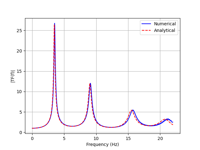
A surface point is located across the distributed files. Its numerical surface-to-base amplification is compared with the same analytical layered profile used for the column example.
The amplified deformation shows uniform horizontal response across the wider domain and propagation through the layered profile. All available partition meshes are rendered in synchronized frames.
Run The Example
The default run builds and exports all eight partitions but does not launch the solver. Parallel execution requires an MPI-enabled OpenSees runtime. To inspect the same domain in forced-serial mode, set:
$env:FEMORA_EXAMPLE_PARTITIONS = "0"
python examples/site_response/partitioned_layered_soil_domain.py
The Colab notebook sets this forced-serial override automatically because the packaged browser runtime is not MPI-enabled. The model geometry, loading, and post-processing remain the same; only distributed execution is disabled.
After execution, the result companion discovers either the single serial file or all MPI partition files through the same filename pattern.
Complete source
# =============================================================================
# Femora: Fast Efficient Meta-modeling for OpenSees-based Resilience Analysis
# Copyright 2026 Amin Pakzad and Pedro Arduino
# Developed at the UW Geotechnical Lab
# SPDX-License-Identifier: Apache-2.0
# =============================================================================

# femora-colab-input: examples/inputs/motions/FrequencySweep.acc
# femora-colab-input: examples/inputs/motions/FrequencySweep.time
# femora-colab-env: FEMORA_EXAMPLE_PARTITIONS=0
# femora-postprocess: examples/site_response/partitioned_layered_soil_domain_postprocess.py

# %% [markdown]
# # Partitioned Layered Soil Domain
#
# Extend the layered soil column to a 10 m by 10 m domain and partition its
# finite-element mesh into eight connected subdomains with METIS. The generated
# Colab notebook uses the same model in forced-serial mode because its packaged
# OpenSees runtime is not MPI-enabled.

# %%
"""Build a partitioned 3D layered site-response model with the current API."""

from __future__ import annotations

import os
from pathlib import Path

from femora import Model, runtime
from femora.utils.paths import motions_dir


OUTPUT_DIR = Path("example_outputs") / "partitioned_layered_soil_domain"
RESULTS_DIR = OUTPUT_DIR / "results"
OPENSEES = os.environ.get("FEMORA_OPENSEES")
NUM_PARTITIONS = int(os.environ.get("FEMORA_EXAMPLE_PARTITIONS", "8"))
PLOT_MODEL = False

DOMAIN_WIDTH = 10.0
DOMAIN_DEPTH = 18.0
HORIZONTAL_ELEMENT_SIZE = 1.0
GRAVITY = 9.81
DYNAMIC_DT = 0.001
DYNAMIC_FINAL_TIME = 40.0

LAYERS = [
    ("dense_ottawa_lower", 145.0e6, 19.9, 2.6, 1.3),
    ("dense_ottawa_middle", 145.0e6, 19.9, 2.4, 1.2),
    ("dense_ottawa_upper", 145.0e6, 19.9, 5.0, 1.0),
    ("loose_ottawa", 75.0e6, 19.1, 6.0, 0.5),
    ("dense_monterey", 42.0e6, 19.8, 2.0, 0.5),
]


# %% [markdown]
# ## Build the three-dimensional profile
#
# The material profile and vertical discretization match the column example.
# Only the horizontal footprint changes: each elevation now contains a 10 by 10
# grid of brick elements.

# %%
OUTPUT_DIR.mkdir(parents=True, exist_ok=True)
model = Model(
    model_name="partitioned_layered_soil_domain",
    model_path=str(OUTPUT_DIR.resolve()),
)
model.set_results_folder(RESULTS_DIR.resolve().as_posix())

damping = model.damping.frequency_rayleigh(
    user_name="soil_damping",
    f1=2.76,
    f2=13.84,
    damping_factor=0.03,
)
soil_region = model.region.element(user_name="soil_domain", damping=damping)

z_bottom = -DOMAIN_DEPTH
layer_names = []
horizontal_cells = round(DOMAIN_WIDTH / HORIZONTAL_ELEMENT_SIZE)

for name, shear_modulus, unit_weight, thickness, element_size in LAYERS:
    density_si = unit_weight * 1_000.0 / GRAVITY
    shear_velocity = (shear_modulus / density_si) ** 0.5
    young_modulus = 2.0 * shear_modulus * 1.3 / 1_000.0
    density = density_si / 1_000.0
    print(f"{name:24s} Vs = {shear_velocity:7.2f} m/s")

    material = model.material.nd.elastic_isotropic(
        user_name=f"{name}_material",
        E=young_modulus,
        nu=0.3,
        rho=density,
    )
    element = model.element.brick.std(
        ndof=3,
        material=material,
        b1=0.0,
        b2=0.0,
        b3=-GRAVITY * density,
    )
    model.meshpart.volume.uniform_rectangular_grid(
        user_name=name,
        element=element,
        region=soil_region,
        x_min=-DOMAIN_WIDTH / 2.0,
        x_max=DOMAIN_WIDTH / 2.0,
        y_min=-DOMAIN_WIDTH / 2.0,
        y_max=DOMAIN_WIDTH / 2.0,
        z_min=z_bottom,
        z_max=z_bottom + thickness,
        nx=horizontal_cells,
        ny=horizontal_cells,
        nz=round(thickness / element_size),
    )
    layer_names.append(name)
    z_bottom += thickness


# %% [markdown]
# ## Partition and constrain the domain
#
# By default, METIS partitions the cell-connectivity graph into eight connected,
# approximately balanced subdomains. Set `FEMORA_EXAMPLE_PARTITIONS=0` to build
# the same model as a forced-serial domain; the Colab setup applies this override
# automatically.

# %%
model.assembler.create_section(
    meshparts=layer_names,
    num_partitions=NUM_PARTITIONS,
    partitioner="metis",
    merge_points=True,
)
model.assembler.assemble(merge_points=True, progress_callback=lambda *_: None)

model.constraint.mp.laminar_boundary(
    bounds=(-DOMAIN_DEPTH + 0.1, 0.0),
    dofs=[1, 2, 3],
    direction=3,
)
model.constraint.sp.fix_macro_z_min(dofs=[1, 1, 1], tol=1.0e-6)


# %% [markdown]
# ## Apply the motion and define the analyses

# %%
motion_directory = motions_dir()
excitation = model.time_series.path(
    filePath=(motion_directory / "FrequencySweep.acc").resolve().as_posix(),
    fileTime=(motion_directory / "FrequencySweep.time").resolve().as_posix(),
    factor=GRAVITY,
)
uniform_excitation = model.pattern.uniform_excitation(
    dof=1,
    time_series=excitation,
)
response_recorder = model.recorder.vtkhdf(
    file_base_name="partitioned_site_response.vtkhdf",
    resp_types=["accel", "disp", "vel"],
    delta_t=0.01,
)

constraint_handler = model.analysis.constraint.transformation()
if NUM_PARTITIONS > 1:
    numberer = model.analysis.numberer.parallelrcm()
    system = model.analysis.system.mumps()
else:
    numberer = model.analysis.numberer.rcm()
    system = model.analysis.system.bandgeneral()
algorithm = model.analysis.algorithm.linear()
test = model.analysis.test.normunbalance(tol=1.0e-8, max_iter=10)
integrator = model.analysis.integrator.newmark(gamma=0.6, beta=0.3025)

gravity_analysis = model.analysis.transient(
    name="gravity",
    constraint_handler=constraint_handler,
    numberer=numberer,
    system=system,
    algorithm=algorithm,
    test=test,
    integrator=integrator,
    dt=1.0,
    num_steps=30,
)
dynamic_analysis = model.analysis.transient(
    name="frequency_sweep",
    constraint_handler=constraint_handler,
    numberer=numberer,
    system=system,
    algorithm=algorithm,
    test=test,
    integrator=integrator,
    dt=DYNAMIC_DT,
    final_time=DYNAMIC_FINAL_TIME,
)

model.process.add_step(gravity_analysis, "Establish gravity")
model.process.add_step(uniform_excitation, "Apply the base excitation")
model.process.add_step(response_recorder, "Record the distributed response")
model.process.add_step(model.actions.set_time(0.0), "Reset pseudo-time")
model.process.add_step(dynamic_analysis, "Run the site-response analysis")


# %% [markdown]
# ## Export the partitioned model
#
# Femora writes one partition-aware Tcl model. Launching an eight-partition
# analysis requires the matching MPI-enabled OpenSees runtime.

# %%
tcl_file = OUTPUT_DIR / "partitioned_layered_soil_domain.tcl"
model.export_to_tcl(
    filename=str(tcl_file.resolve()),
    progress_callback=lambda *_: None,
)

core_ids = model.assembled_mesh.cell_data["Core"]
print("\nPartitioned layered soil domain")
print(f"  Nodes:       {model.assembled_mesh.n_points}")
print(f"  Elements:    {model.assembled_mesh.n_cells}")
print(f"  Core IDs:    {sorted(set(int(value) for value in core_ids))}")
print(f"  Tcl model:   {tcl_file.resolve()}")

if NUM_PARTITIONS == 0 and OPENSEES is not None:
    runtime.run(tcl_file, executable=OPENSEES, cwd=OUTPUT_DIR.resolve())
    print("  Solver:      completed")
elif NUM_PARTITIONS > 1:
    print("  Solver:      not launched (run with an MPI-enabled OpenSees runtime)")
else:
    print("  Solver:      not run (set FEMORA_OPENSEES to run OpenSees)")


# %% [markdown]
# ## Optional visualization

# %%
if PLOT_MODEL:
    model.assembler.plot(show_edges=True, scalars="Core")